A Brief Overview of ADMM
The alternating direction method of multipliers (ADMM) has emerged as an important algorithm for convex optimization. Here are some of my notes on how it works. If this piques your interest, I highly recommend you watch this lecture by Stephen Boyd, the OG of ADMM (slides here).
As Boyd puts it: “The alternating direction method of multipliers (ADMM) is an algorithm that solves convex optimization problems by breaking them into smaller pieces, each of which are then easier to handle.”
We will consider the problem
where and are convex.
Many practical problems can be written this way. Frequently, is smooth and easy to minimize, and is a rule or a penalty: e.g. keep inside a set, constrain most entries to be zero, keep a matrix positive semidefinite.
How ADMM Works
The way ADMM works is to introduce a dual variable , with one entry per row of the constraint, and a penalty parameter . Then we iteratively update , , and . At each iteration we do the following:
The x-step. Fix and and minimize over alone. We consider and not .
The z-step. The same thing for , using the we just computed. Now we consider and not .
The y-step. Now we update using whatever is left of the constraint violation. We scale it by .
As Boyd notes, you can think of as a vector of prices for violating the constraint . In the x-step, is the focus, but we pay the current price for the “x share” of the violation, plus a quadratic penalty. In the z-step, does the same. In the y-step, we raise the price wherever the constraint is still violated. Note that stops changing only when .
In certain cases it’s far, far easier to solve these subproblems, as compared to the original problem. And sometimes we can monitor our progress and stop when we have a “good enough” solution. These properties can make ADMM a very desirable approach in many cases.
So let’s take a step back and walk through how we derive the approach above. Then we will go through an example.
Derivation
The first step is to form the Augmented Lagrangian:
The first three terms are the usual Lagrangian. The last is the “augmented” part. It is zero at every point that satisfies the constraint, so it does not change the solution. What it buys us is subproblems that behave well even when and are not strictly convex, which is exactly the situation when is a rule like “stay inside this set.” This is basically the “good news” on Boyd’s slide 11.
The older method of multipliers minimizes over and together, then raises the price of violating the constraint: . The problem with this is that it’s hard to minimize over both together: that’s what we wanted to avoid in the first place. This is why in ADMM we break it up: minimize over , then over , once each, and update right away. This going back and forth is the “alternating direction” part.
There are more details but I will refer you to the slides or the talk if you are interested. The point is that ADMM converges to the optimal value under reasonable conditions. It’s good for situations where you want to get pretty good accuracy on big problems.
Example
Claude came up with a great example, so here we go. Let’s find the lowest point of a tilted bowl inside a box. The bowl is
and the box is , . The bottom of the bowl is at , which is outside the box. The obvious guess is the point of the box closest to , which is . That guess is wrong. The off-diagonal entries of tilt the bowl, and sliding up the wall to lowers from to .
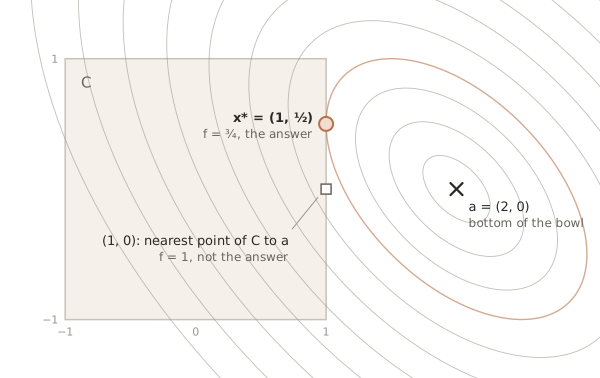
Writing it in ADMM form
Let be the function that is inside the box and outside. Then our problem is to minimize . Give its own copy of the variable (), and require the copies to match:
That is our template with , , and . Neither piece is hard by itself, which is why ADMM is great for this example.
The three steps
Plug , and into the steps from before.
The x-step. We minimize . This is quadratic, so set the gradient to zero: . That gives
a 2 × 2 linear solve: easy.
The z-step. We minimize . Completing the square, this is the same as minimizing
TL;DR: find the point of the box closest to . For a box that means clipping each coordinate to :
The bowl is nowhere to be seen.
The y-step.
Running it
Take and start from . The first iteration can be done by hand:
- x-step: solve , so . This is outside the box.
- z-step: clip to get .
- y-step: .
Here is how it continues:
| 1 | (1.2500, 0.2500) | (1, 0.2500) | (0.2500, 0) | 0.25 |
| 2 | (1.5000, 0.2500) | (1, 0.2500) | (0.7500, 0) | 0.50 |
| 3 | (1.3125, 0.3125) | (1, 0.3125) | (1.0625, 0) | 0.31 |
| 5 | (1.1094, 0.4219) | (1, 0.4219) | (1.3594, 0) | 0.11 |
| 10 | (1.0059, 0.4951) | (1, 0.4951) | (1.4932, 0) | 0.0059 |
| 20 | (1.0000, 0.5000) | (1, 0.5000) | (1.5000, 0) | 0.00001 |
In the second iteration actually moves farther outside the box. The x-step still wants the bottom of the bowl, and a price of 0.25 is not nearly enough to talk it out of that. So the y-step raises the price again, and again, each time by the amount still overshoots the wall. Meanwhile stays on the wall and slides up it. After 24 iterations both residuals are below .
You can step through it yourself:
- x
- –
- z
- (0.0000, 0.0000)
- y
- (0.0000, 0.0000)
- Primal residual ‖x − z‖
- –
- Dual residual ρ‖z − z_prev‖
- –
Example in Python
import numpy as np

Q = np.array([[2.0, 1.0], [1.0, 2.0]])
a = np.array([2.0, 0.0])
rho = 1.0
z = np.zeros(2)
y = np.zeros(2)

for k in range(1, 25):
    x = np.linalg.solve(Q + rho * np.eye(2), Q @ a + rho * z - y)  # x-step: a linear solve
    z_prev = z
    z = np.clip(x + y / rho, -1, 1)                                # z-step: clip to the box
    y = y + rho * (x - z)                                          # y-step: reprice
    r = np.linalg.norm(x - z)                                      # primal residual
    s = rho * np.linalg.norm(z - z_prev)                           # dual residual
    print(k, x, z, y, r, s)
In future posts, I will apply ADMM to an old friend: QAP.